A Model of Good Practice for Machine Learning in Remote Sensing

In remote-sensing machine learning, the difficult question is rarely whether a model can be trained. The harder question is whether its predictions remain scientifically credible and geographically transferable under the combined constraints of limited samples, complex surface processes, and spatial heterogeneity.

Remote-sensing retrieval problems often combine sparse field samples, high-dimensional spectra, weak target responses, and strong background interference. Without explicit process constraints and a rigorous validation design, a flexible machine-learning model can mistake local correlation for stable structure. The result may look accurate in conventional validation while failing when it is transferred into genuinely unsampled space.

Sun et al. recently published CIDA: A context-informed decoupling approach for soil trace element estimation using spaceborne cross-sensor data in the ISPRS Journal of Photogrammetry and Remote Sensing. The paper addresses a structural imbalance that is common in small-sample remote-sensing retrieval: sparse field measurements on one side, and a high-dimensional spectral feature space on the other.

The authors propose Context-Informed Decoupling Analysis (CIDA), a framework that interprets the indirect spectral expression of trace elements such as Zn and Cu under soil-geochemical constraints and reduces the risk of overfitting in small-sample machine learning.

Among applied remote-sensing machine-learning papers I have read, this is one of the most technically disciplined examples. Its strength is not a novel model architecture. It is the clarity with which it limits what the model is allowed to do: learning is constrained by geochemical process knowledge, performance is tested under spatial extrapolation, and interpretation is pushed beyond feature ranking toward the structure of the mechanism represented by the model.

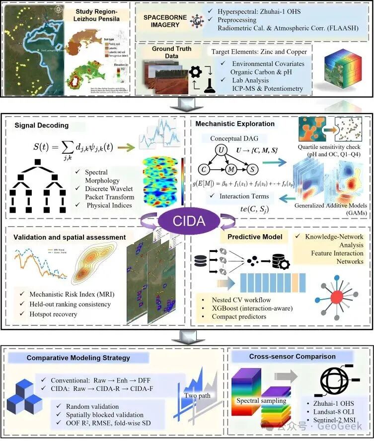
Figure 1 · CIDA workflow: a disciplined modelling path for small-sample remote-sensing machine learning. Instead of sending high-dimensional spectral features directly into a predictive model, CIDA first introduces soil-geochemical context and reorganizes the relations among spectral features, environmental variables, and target elements. The aim is to reduce overfitting when samples are sparse (Sun et al., 2026, Fig. 2).

01 · Context-aware and mechanism-guided learning: what should the model learn?

Core point: the spectral relation to the target is not fixed. It changes with background conditions. A model should not search high-dimensional feature space without process constraints.

A common assumption in remote-sensing machine learning is that the relation between remote-sensing predictors and a target variable is a static, homogeneous mapping that a sufficiently flexible model can approximate automatically. In data-rich problems with direct signals, that assumption can work reasonably well: enough observations can statistically suppress many accidental correlations in a large feature space.

The situation changes in small-sample, weak-signal, heterogeneous retrieval. Model freedom can greatly exceed the information content of the data. The training data alone cannot constrain the search space strongly enough. Without additional structure, the model can capture chance correlations in high-dimensional space and produce the familiar pattern of high training or random-validation accuracy with weak transfer to new areas.

Soil trace elements such as Zn and Cu make the problem concrete. They are not classic strong spectral targets. A satellite usually does not record a clean absorption feature caused directly by metal concentration. Instead, the signal reflects the combined influence of soil organic carbon, pH, mineral composition, iron oxides, clay, moisture, and other properties.

The remote-sensing signal is therefore not a direct projection of the target element. It is an integrated expression of the soil system. The central modelling problem is not only that the target signal is weak. It is that the signal is mixed: is the model learning information about the element, or is it learning environmental variables that happen to act as proxies under the local background?

This is not unusual in remote sensing. Nutrients such as total nitrogen and total phosphorus in water are not generally direct optically active constituents; their retrieval often depends on indirect optical responses created by Chl-a, suspended matter, CDOM, turbidity, and hydrodynamic conditions. Soil-salinity retrieval is likewise modulated by moisture, texture, surface roughness, and vegetation cover.

For weak-response or indirectly expressed targets, a machine-learning model has to answer a scientific question before it answers a predictive one: is it learning the target, or an environmental proxy for the target?

This is where CIDA becomes important. It does not begin by feeding all spectral variables into a predictive model. It begins by acknowledging context dependency. The same spectral feature can be strongly related to Zn or Cu under one combination of pH and organic carbon, weak under another, reversed under a third, or irrelevant altogether.

This instability of proxies is a general problem in applied remote sensing; I discuss the broader structure in What Remote Sensing Sees—and What It Does Not: The Proxy-of-a-Proxy Problem.

CIDA is therefore not ordinary feature engineering. It is a strategy for decoupling and organizing relations under geochemical context. Variables such as pH and organic carbon enter feature selection and relation learning so that the model does not decide which spectral information matters independently of the soil environment.

In effect, domain knowledge compresses the nominally data-driven search space into a geochemically plausible subspace. The model still learns, but it does not learn blindly.

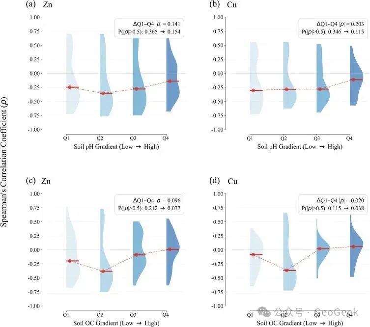
Figure 2 · Context dependency: regulation of metal–spectral correlation structure by pH and organic carbon. The distributions of correlations between spectral features and Zn/Cu are compared across pH and OC quartile groups. The relationships are not static; they change with the geochemical background (Sun et al., 2026, Fig. 5).

02 · Spatial validation: is what the model learned transferable?

Core point: a high R² under random validation does not demonstrate spatial extrapolation. Spatially blocked validation is the more relevant test of geographic generalization.

Remote-sensing mapping differs fundamentally from ordinary tabular prediction because the output is ultimately projected into geographic space. Geographic samples are not independent. Nearby samples tend to share land-surface conditions, soil background, and sampling history.

Conventional random cross-validation can ignore exactly this structure. Random assignment can place neighboring samples in both the training and validation sets. The nominal validation data are then not geographically independent of the training data. A model can exploit spatial proximity, local background similarity, or sampling structure rather than learn a soil–spectral relation that transfers.

I discussed this issue in What Nature and Science Papers Reveal about Extrapolation Risk at Global Scale: information leakage created by spatial autocorrelation can substantially inflate model performance, and many studies underestimate the problem.

The CIDA paper addresses it directly by reporting both random out-of-fold validation and spatially blocked out-of-fold validation. The two tests answer different questions.

Random validation tests statistical fitting capacity: can the model extract a predictive signal from a mixed sample? Spatially blocked validation tests geographical transferability: does the model remain useful in spatially independent regions?

For remote-sensing mapping, the second question is closer to the task that matters. Mapping is inference from finite samples into unsampled space, and every such extrapolation is a test against spatial heterogeneity.

Does CIDA generalize better than conventional strategies? The comparison is informative. Conventional approaches—direct spectral modelling, spectral enhancement, and feature fusion—differ in detail but share a tendency to accumulate features and allow the model to search among them. They can perform well under random validation and then degrade strongly under spatial blocking.

CIDA reorganizes the feature structure under contextual constraints before the prediction stage and remains more stable under spatial transfer. The difference is methodological: conventional workflows ask the model to discover structure in a high-dimensional space; CIDA uses domain knowledge to reduce the space before learning begins.

This is also a bias–variance trade-off. With few samples, variance can dominate error. A controlled amount of mechanistic bias can be safer than allowing an unconstrained model to fit every idiosyncrasy of the training set. In small-sample remote-sensing retrieval, reducing variance through scientific constraints is often preferable to maximizing in-sample flexibility.

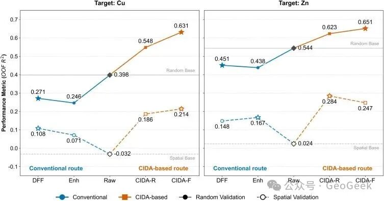
Figure 3 · Conventional strategies versus CIDA: model comparison should not stop at random-validation accuracy. CIDA improves not only predictive scores but also robustness under small samples, high-dimensional features, and complex soil background by using mechanistic constraints and feature compression (Sun et al., 2026, Fig. 9).

How much of random-validation performance actually transfers?

The paper further introduces spatial performance retention, defined as the ratio between R² under spatially blocked validation and R² under random validation. The metric asks a useful question: how much of the apparent skill under random validation survives when the model moves from explaining known spatial structure to predicting unknown space?

Some performance decline under spatial blocking is expected. What matters is its magnitude. If a model is excellent under random validation and collapses once spatial independence is imposed, much of the original R² may have come from local spatial structure or high-dimensional chance correlation. A model that remains comparatively stable under a stricter spatial partition is closer to the reliability needed for mapping.

The paper extends the comparison across sensor combinations. Under CIDA, spatial performance retention is higher than under conventional strategies across those combinations, providing additional evidence that process constraints improve geographic generalization rather than merely in-sample fit.

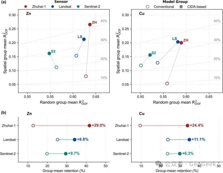
Figure 4 · Spatial stability and cross-sensor performance. Different sensor combinations and model groups are compared for Zn and Cu retrieval, and group-mean retention measures how much predictive structure remains under spatial blocking relative to random validation. The metric tests geographic transfer more directly than reporting random R² alone (Sun et al., 2026, Fig. 11).

What if accurate pixel-level extrapolation is not achievable?

Spatial validation also reveals a practical limit. Under small samples, weak signals, and strong heterogeneity, high-accuracy extrapolation of absolute concentration at every pixel may simply be unrealistic.

In that setting, promising that “every pixel is accurate” is neither necessary nor scientifically defensible. For environmental management, the model may be more valuable if it can identify stable patterns, trends, hotspots, and priority areas than if it produces a seemingly precise concentration at every location.

This is the role of the paper's Mechanistic Risk Index (MRI). It shifts evaluation from concentration regression alone toward hotspot and priority-area identification. Spatial-consistency analysis asks whether the model can identify where additional sampling, monitoring, or intervention should be prioritized.

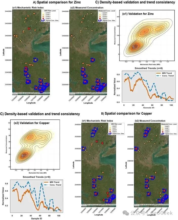
Figure 5 · Spatial agreement between MRI and high measured Zn/Cu samples. Density distributions and trend lines compare the Mechanistic Risk Index with observed concentration gradients. In small-sample soil remote sensing, stable identification of hotspots, high-risk zones, and priority survey areas may be more useful for management than unstable claims of pixel-perfect concentration (Sun et al., 2026, Fig. 8).

03 · Mechanistic interpretability: from feature attribution to knowledge structure

Core point: interpretability should not end with a ranking of feature contributions. It should ask whether the model has organized information in a way that is coherent with process knowledge.

A second common problem in remote-sensing machine learning is the reduction of “interpretability” to SHAP or feature-importance plots. SHAP is useful. It can quantify the marginal contribution of features to model output, compare variable importance, and reveal nonlinear response structure in an otherwise opaque model.

But SHAP is still a post-hoc attribution method. It answers “which features contribute more?” It does not by itself answer whether those contributions form a mechanism consistent with process knowledge, or whether the same contribution structure transfers geographically. For the epistemic boundary of SHAP, see The Interpretive Boundary of SHAP: From Model Attribution to Causal Identification.

One of the strongest aspects of the CIDA paper is that it moves beyond single-feature attribution toward structured mechanistic interpretation. The authors use knowledge networks to show how interaction terms, soil-chemical constraints, and spectral features are organized differently for Zn and Cu in the best CIDA models.

Traditional SHAP takes a feature as the unit of explanation and asks what the model used. The knowledge-network view asks a different question: how are variables organized through the geochemical background into a coherent structure? The first identifies contributions; the second seeks an interpretable organization of those contributions.

The resulting structures differ for Zn and Cu. Zn prediction is more concentrated, with interactions involving organic carbon playing a stronger organizing role. Cu is more distributed, with pH, organic carbon, and multiple spectral features participating jointly.

Those differences are not interpreted as mere algorithmic artifacts. They are broadly consistent with known differences in soil occurrence, adsorption, complexation, and environmental regulation of Zn and Cu. At that point the model becomes more than a device for outputting a concentration estimate. It becomes a tool for thinking about how different elements are expressed indirectly through spectra under different soil backgrounds.

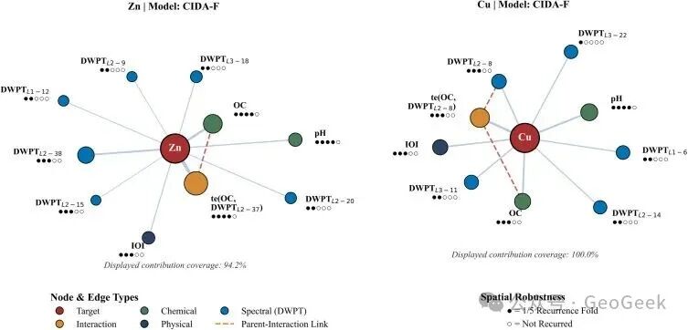
Figure 6 · Mechanistic interpretability beyond SHAP: from feature attribution to knowledge networks. The best CIDA models organize soil-chemical variables, interaction terms, and spectral features into different explanatory structures for Zn and Cu. The question is no longer only which feature contributes most, but how the variables form an interpretable structure (Sun et al., 2026, Fig. 10).

Closing note

I regard this paper as an unusually disciplined example of machine learning in applied remote sensing for three reasons.

First, it accepts that spectral-feature–metal-concentration relationships are neither stable nor homogeneous. They are modulated by geochemical context such as pH and organic carbon. Feature learning is therefore constrained by context-aware, mechanism-guided learning rather than unconstrained high-dimensional search.

Second, it accepts that random validation does not demonstrate mapping ability. Spatially blocked out-of-fold validation, spatial performance retention, and hotspot-consistency validation are used to test the geographic transfer required for inference into unsampled space.

Third, it accepts that predictive performance is not the same thing as scientific understanding. Interpretation is pushed beyond feature attribution toward something closer to knowledge-structure understanding.

George Box's familiar line remains useful: “All models are wrong, but some are useful.” A model is not a mirror of the world. It is a limited mapping of it. The important question is not how impressive an accuracy score looks in isolation, but whether we understand the boundary within which the model is valid, the conditions under which it fails, and what value remains after that failure.

The strength of this paper is that it does not evade the most difficult parts of applied remote sensing: small samples, weak target signals, background coupling, and spatial extrapolation. It acknowledges those constraints and then designs the workflow around them.

Admitting what is unknown is not a retreat from science. It is the beginning of finding out. In a literature saturated with “better accuracy” and “SOTA,” a clear statement of what the model cannot yet know is often more scientifically valuable than another confirmation of what it already fits.