Stress-Testing AlphaEarth in Agriculture

Harvesting AlphaEarth, a collaboration between David B. Lobell's group at Stanford and Corteva, is not another agricultural remote-sensing model. It places Google DeepMind's AlphaEarth Foundation (AEF) in a demanding application domain and asks whether it is actually ready to function as an off-the-shelf geospatial foundation representation for agriculture.

The paper's main conclusion is clear. AEF performs strongly when training and application remain local, and it is already competitive for tasks such as crop-yield prediction and county-scale tillage mapping. But its advantage diminishes rapidly when the task requires transfer across regions or scales, or when the target is highly time-sensitive.

The value of the study lies less in asking which model is “more accurate” than in making three agricultural requirements explicit in the evaluation of AEF: generalizability, time sensitivity, and interpretability.

01 · From general-purpose advantage to conditional advantage in agriculture

To understand the benchmark, it helps to return to the aim of the original AEF paper. Earth observation carries a persistent feature-engineering burden: heterogeneous data sources, inconsistent spatial and temporal resolution, sparse and asynchronous observations, and substantial harmonization work across sensors.

AEF addresses this by compressing multimodal information—including optical and radar imagery, LiDAR, climate, topography, gravity, and text—into a unified 64-dimensional embedding space. Annual global representation layers at 10 m resolution are released for 2017–2024 and can be accessed directly in Google Earth Engine.

Harvesting AlphaEarth briefly reviews this design and notes an important gap in the original evaluation. Most internal AEF benchmarks focused on tasks such as land use and land cover. Agriculture places much greater demands on narrow temporal windows, transfer across spatial scales, and spatial generalization, so the evidence for agricultural use remained incomplete.

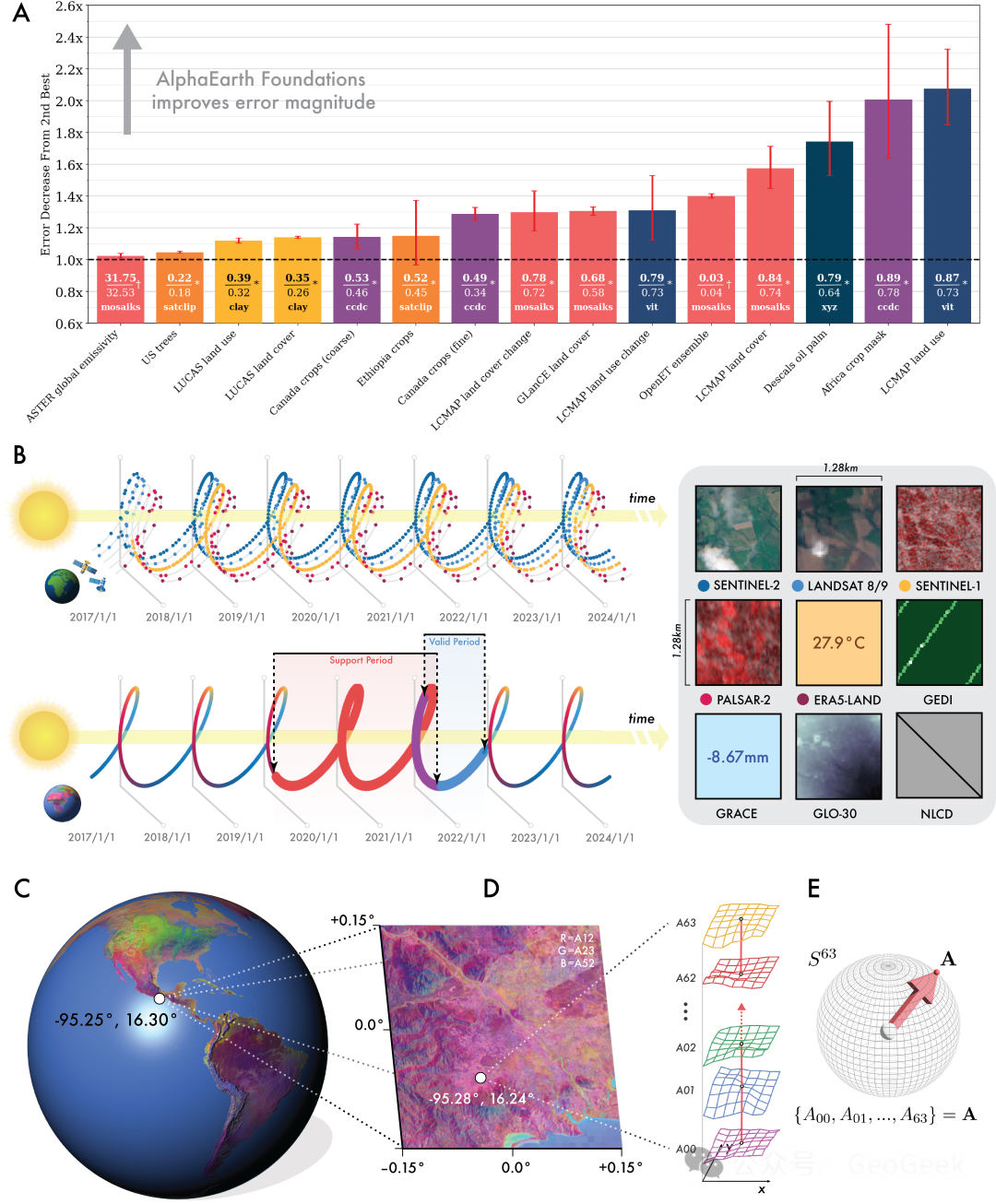
Figure 1 · The original AEF paper reported strong performance of AlphaEarth embedding fields across multiple downstream tasks.

The real question in Harvesting AlphaEarth is therefore not whether AEF is useful. It is how far its usefulness extends once agricultural constraints become explicit.

The study evaluates three downstream tasks: crop-yield prediction, spring tillage mapping, and cover-crop mapping. It tests both county and field scales, combining public USDA-NASS data with proprietary field-level data from Corteva. The field-yield dataset alone includes 89,938 maize fields, 73,492 soybean fields, and 20,401 winter-wheat fields; the cover-crop dataset contains 47,709 field-years.

A particularly useful design choice is the baseline. The authors do not compare AEF only against other foundation models. They compare it with remote-sensing feature workflows that agricultural researchers actually use. The resulting claims are therefore closer to a real methodological choice in research or production.

The evaluation protocol is also stricter than many demonstrations of model utility. Random splits, which would exaggerate performance under spatial autocorrelation, are avoided. State-Year and County-Year cross-validation reduce spatial leakage; Yearly CV tests cross-year generalization; and separate Scale-Transfer and Space-Transfer experiments test transfer across spatial support and ecological regions.

The benchmark is asking a practical question: if prediction does not remain in the same region, at the same scale, and in adjacent years, does AEF still retain the advantage reported in broad foundation-model benchmarks?

02 · AEF is not merely a proof of concept

Under local training and application, AEF performs well.

For county-level yield prediction, AEF-based and conventional remote-sensing models are broadly comparable under State-Year CV. Under Yearly CV, which more closely resembles a real cross-year prediction setting, AEF is more stable. With XGBoost, county-level Yearly-CV scores for maize, soybean, and winter wheat are 0.77, 0.77, and 0.78, respectively, compared with 0.74, 0.70, and 0.69 for the RS-XGB baseline.

The difference is more than a small numerical gain. In a split where training and testing are separated by year and the model cannot rely on similarity between neighboring years, annual AEF embeddings still retain substantial information about crop condition. For winter wheat in particular, the paper reports that RS-based models tend to underpredict the high-yield range, while AEF partly reduces that bias.

At county scale, AEF has therefore moved beyond “worth trying.” It is already a plausible substitute for part of a conventional feature-engineering workflow.

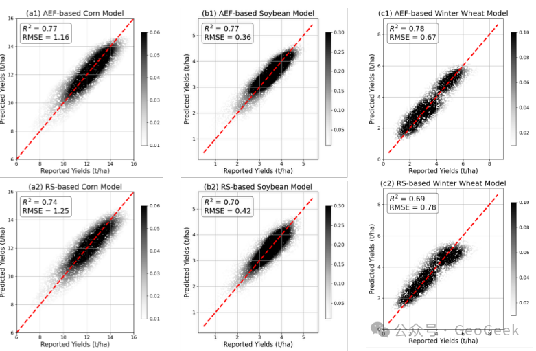
Figure 2 · Observed and predicted county-level yields for three crop types under Yearly CV.

This performance is not achieved against a weak baseline. The RS baseline is a mature, task-specific agricultural representation. For yield prediction it includes six Landsat bands, NDVI, GCVI, monthly climate variables, second-order harmonic regression and phenological metrics that compress the growing-season time series into 80 harmonic/phenology predictors, plus monthly growing degree days and precipitation.

AEF therefore remains competitive against a conventional workflow that has already incorporated substantial agronomic and remote-sensing knowledge. In practical terms, an off-the-shelf foundation representation is approaching the performance of a carefully engineered domain workflow.

Tillage mapping points in the same direction. At county level, prediction of the proportion of low-intensity tillage is similar between AEF and RS; aggregated across years, AEF-RF is slightly higher than RS-RF but the difference is modest. At field level under County-Year CV, model accuracies and weighted F1 scores are generally around 0.75–0.80, with AEF remaining competitive.

This makes AEF a realistic option for the common “local training, local deployment” agricultural setting.

There is also a data-engineering advantage. The paper highlights three practical benefits: multisource harmonization is built into the representation; AEF is hosted as an image dataset in GEE and can be accessed without the usual pipeline of scene downloading, cloud masking, temporal alignment, and feature fitting; and spatial coverage is more complete.

One example is revealing. Of 90,210 maize-field yield records, AEF embeddings were available for nearly the full set, while conventional RS features could be successfully constructed for only 89,938. Most losses came from insufficient Landsat temporal coverage or failure of harmonic fitting. For agricultural researchers, AEF's value is therefore not only predictive performance. It can materially reduce data-preparation cost and the barrier to entry.

03 · The boundaries of applicability

The paper's more important result is that the questions agriculture cares about most are also where the current AEF product is weakest.

The first boundary is scale transferability. In the Scale-Transfer experiment, models are trained at county scale and tested on field-scale yield. AEF performs substantially worse than conventional RS features. For maize, AEF-XGB scores 0.25 compared with 0.38 for RS-XGB; for soybean, 0.11 versus 0.24; for winter wheat, AEF-XGB falls to −0.04 while RS-XGB remains at 0.22.

The authors offer a direct explanation. An embedding is a compressed representation. Once it is aggregated to a county mean, within-county heterogeneity that is strongly related to field-level yield is diluted. Conventional RS features still retain more direct physical information about canopy structure, vegetation vigor, and soil moisture, which transfers more reliably across scales.

This result matters beyond the benchmark. A unified foundation representation does not automatically imply robustness to scale. In agriculture, scale is not an incidental technical choice. It determines whether the information carried by a variable remains valid for the target process. An embedding useful as a county average may no longer represent field-level differences in crop growth.

The experiment therefore corrects a common expectation: a high-level pretrained representation is not inherently better for cross-scale transfer than lower-level physical features.

The second boundary is time sensitivity. This is especially clear in tillage and cover-crop mapping.

For field-level tillage classification under Yearly CV, accuracy and weighted F1 of AEF-based models fall to about 0.70, while RS-based models remain closer to 0.75. High-intensity tillage is difficult because its signal exists within a short phenological window: residues are removed and the soil surface is disturbed, and the contrast is most visible only for a limited period.

The RS workflow organizes bands, vegetation indices, and tillage indices monthly from April through June. The public AEF product is an annual embedding. Even though AEF training emphasizes “continuous time-series featurization,” the representation users actually access is aggregated at yearly resolution. That temporal support is poorly matched to short-lived agricultural management signals.

Cover-crop mapping makes the problem even clearer. A cover crop spans harvest in one year and planting in the next, so the authors have to concatenate AEF embeddings from two calendar years. The RS baseline instead uses monthly bands, vegetation indices, temperature, and precipitation from October through the following May.

Under both County-Year CV and Yearly CV, RS-based Random Forest is the strongest overall model, with accuracy and weighted F1 around 0.80–0.85. AEF is more sensitive to the positive class—that is, fields with cover crops—but is also more likely to label negative fields incorrectly as positive. The paper also notes that XGBoost performs worse than Random Forest in this task, partly because observations in late winter and early spring are noisy and RF is more robust to that noise.

The implication is important: when observation conditions are poor and the phenological window is narrow, AEF does not show a clear robustness advantage over conventional features.

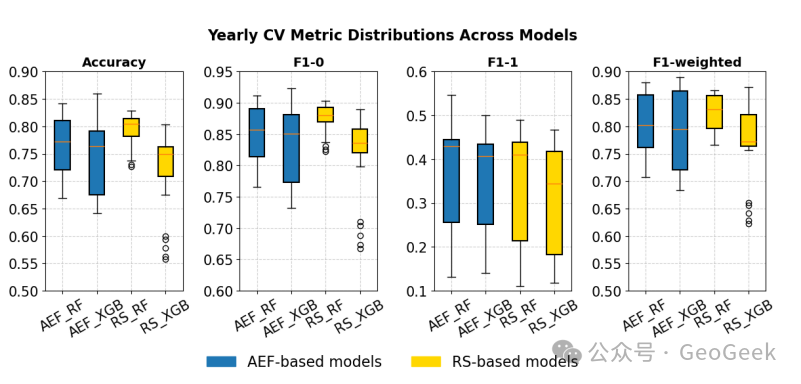
Figure 3 · Interannual variation and model differences in field-level cover-crop classification under Yearly CV.

The benchmark therefore separates two ideas that are easy to conflate. A model can have a training architecture that is time-continuous without producing a user-facing representation that is sufficiently time-resolved for the target application. As long as the released product is annual, AEF remains fundamentally limited for within-season forecasting, short-duration management-event detection, and phenological transitions.

04 · Spatial transfer can fail

If scale and timing reveal local boundaries, the space-transfer experiment gives a deeper warning: AEF is not yet an agricultural representation that can be expected to work independently of regional context.

The paper divides the US Corn Belt into two ecological regions, the Eastern Temperate Forests (ETF) and the Great Plains (GP), and performs transfer in both directions.

The county-level yield results are striking. For maize transferred East→West, AEF-based RF scores only 0.02 while RS-based RF reaches 0.66. For soybean East→West, AEF-based RF falls to −0.28 while RS-based RF remains at 0.53. At field level, AEF still trails the RS baseline, although the gap is smaller.

AEF can therefore match or outperform conventional features in local fitting while losing that advantage rapidly once training and application regions are separated.

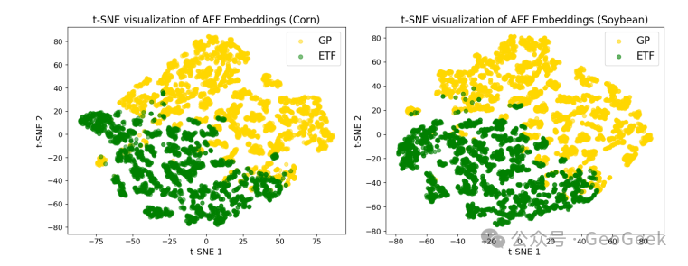
Figure 4 · County-level crop-specific AEF embeddings from different ecological regions separate clearly in two-dimensional t-SNE space.

This visualization is one of the paper's most informative results. Crop-specific embeddings from the eastern and western regions occupy distinct parts of embedding space, with only limited overlap near the regional boundary. The plot connects performance failure to representation structure: AEF is not encoding only a transferable “crop state.” It also contains strong regional specificity.

A model trained in one region therefore learns not simply that a representation corresponds to a particular yield, but that a region-specific representation corresponds to that yield. Transfer becomes difficult by construction.

The authors push the test beyond the United States. A county-level soybean model trained in the US is used to predict Argentine soybean yields during 2019–2024. AEF fails badly in every year; pooled scores for RF and XGB are −2.13 and −2.45. Conventional RS models are far from perfect but remain positive at 0.27 and 0.26.

This is not a minor regional shift within the Corn Belt. It is a structural failure under cross-country transfer.

The discussion of why is as important as the result. The authors suggest two possible mechanisms. First, AEF is trained not only to reconstruct satellite imagery but also DEM and gravity-field information. Those are geographically stable and region-specific signals, which may encourage the embedding to encode location strongly. Second, AEF uses contrastive learning between geolocated Wikipedia text and visual representations. The text naturally contains region-specific information, and multimodal alignment may reinforce geographic identity further.

The lesson is broader than AlphaEarth: multimodality does not automatically increase spatial invariance. It can, in some settings, write regional labels more deeply into the representation.

05 · Agriculture needs explanation as well as prediction

The paper finally asks whether AEF embeddings are interpretable enough for agricultural science.

In county-level maize-yield prediction, feature importance from the conventional RS-based Random Forest tells a scientifically legible story. Satellite features matter more than climate variables; GCVI is more useful than NDVI or raw bands, pointing toward the importance of nitrogen status and chlorophyll-related information in the prediction. Such information can guide feature selection, observation design, and monitoring priorities.

In the AEF-based RF, by contrast, the most important dimensions are A05 and A17. Those labels carry no obvious physical meaning. The most important embedding dimensions also differ markedly between maize and soybean, making it difficult to derive a stable agricultural interpretation.

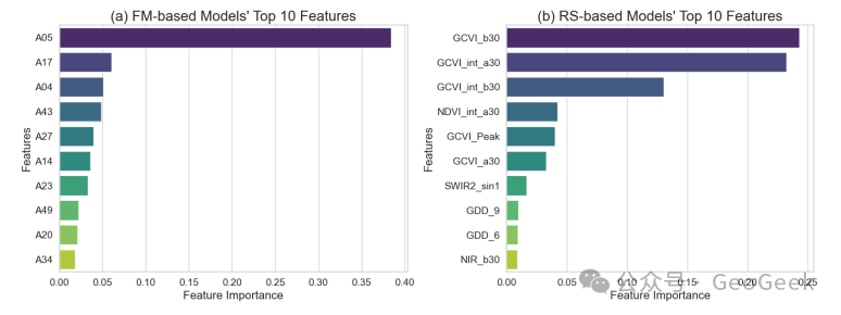
Figure 5 · Feature-importance comparison between AEF dimensions and conventional RS features for county-level maize-yield prediction.

This is not a secondary concern. In agriculture and geoscience, the main scientific question is often not whether prediction can be improved by another few percentage points. It is what information the model relies on, which processes matter, which differences are driven by management, and which reflect environmental background.

AEF currently offers a representation that is highly compressed and easy to use but comparatively difficult to interpret. For rapid predictive modelling, that may be enough. For causal analysis, mechanistic attribution, or management strategy, conventional physical features remain difficult to replace.

The original AEF paper emphasized broad benchmark performance. Harvesting AlphaEarth shows that agricultural value has to be judged along three additional dimensions: whether a representation transfers reliably, whether it resolves the time windows that matter, and whether its information content can be interpreted.

Closing note

The benchmark moves AEF from the category of “powerful general representation” into a more useful one: an agricultural representation with identifiable conditions of validity.

It corrects a tempting but unsupported assumption: that a foundation model will naturally outperform conventional remote-sensing features if it is large enough, trained on enough data, and multimodal enough. In agriculture, scale match, temporal resolution, and regional specificity matter at least as much as model size.

The paper's value is therefore not merely that it lists shortcomings. It points directly to design requirements for the next generation of geospatial foundation models in agriculture: release monthly or seasonal embeddings rather than only annual products; balance geographic sampling more systematically during training to reduce geographic shift; and develop stronger attribution methods so that embeddings become not only usable but interpretable.

Those proposals grow directly out of the experiments. Harvesting AlphaEarth is best read as a boundary-setting paper for both agricultural remote sensing and foundation-model research. It does not dismiss AEF's potential. It shows that progress in a spatiotemporally sensitive domain will require more than a better benchmark score: the representation has to become transferable, interpretable, and deployable at the scale and time support of the actual agricultural process.