Extrapolation Risk in Global-Scale Studies

A few days ago I wrote about the controversy surrounding Bastin et al.'s 2019 Science paper, The global tree restoration potential. The underlying question was simple: when a global map looks complete, precise, and immediately useful for policy, is its evidence base really strong enough to support the global claim being made?

I proposed a basic three-part test for any global map: are the input data reliable, is model validation rigorous, and are the boundaries of extrapolation made explicit?

If we widen the view from one highly influential Science paper to several recent papers in Nature and Science, the same problem appears repeatedly. High-profile global-change research is increasingly good at turning local observations into global narratives: tens of thousands of soil samples become a map of global biodiversity hotspots; training data from limited regions become a continuous global ecosystem map; proxy relations validated over the modern satellite era are extended backward to reconstruct environmental change across half a century.

Methodologically, these studies often face two kinds of representation mismatch.

The first is spatial representativeness mismatch: the training data cover only part of global environmental space, while the model produces a continuous global surface. The second is temporal representativeness mismatch: a recent proxy or empirical relation is transferred into earlier decades, or heterogeneous time series with different start dates and durations are aggregated into a statement about “global long-term change.”

The first creates spatial extrapolation fragility. The second creates a risk of temporal over-interpretation.

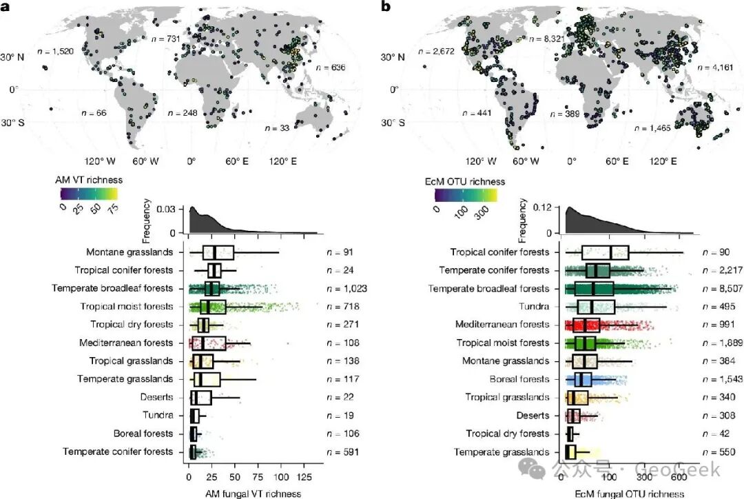
Figure 1 · Sample distribution comes before global prediction. Van Nuland et al. (2025, Nature) show the sample locations used in their global analysis of mycorrhizal fungal richness and richness trends across biomes. The first question for a global conclusion is not how detailed the map looks, but whether the samples adequately represent global environmental space.

01 · Spatial extrapolation risk

A useful example is Van Nuland et al. (2025), Global hotspots of mycorrhizal fungal richness are poorly protected. The study trained machine-learning models on roughly 25,000 georeferenced soil samples and produced global 1 km² maps of mycorrhizal fungal richness and rarity hotspots.

The problem is not that 25,000 samples is a small number. It is that their spatial distribution is uneven. The paper and Extended Data explicitly note that sampling is concentrated in North America, Europe, and Asia. The main map cross-hatches regions described as “underrepresented by the training data (highly extrapolated)” and instructs readers to interpret them cautiously.

More importantly, performance drops sharply between random cross-validation and more demanding spatial validation. For richness models, AM R² falls from 0.61 to 0.20 and EcM from 0.63 to 0.28. For the AM rarity model, kNNDM R² is even −2.55. One of the most important results in the paper, therefore, is not simply where the hotspots are. It is that a substantial fraction of the global hotspot surface is produced under strong extrapolation.

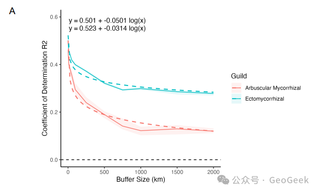
Figure 2 · Model performance declines under spatially independent validation. Supplementary Fig. 3 of Van Nuland et al. (2025) shows R² falling as the buffer size increases in spatially buffered leave-one-out cross-validation.

The lesson is easy to miss. High random-cross-validation accuracy does not automatically imply reliable prediction in unfamiliar regions. I discussed the same issue in the earlier note on Bastin et al. using the analysis of Ploton et al. (2020): when training and test observations are not spatially independent, spatial autocorrelation can systematically inflate apparent model skill.

Van Nuland et al. actually build part of this criticism into their own evaluation. They provide spatial validation alongside random validation. For that reason, the paper is a useful teaching case rather than an example of a study that simply “did validation wrong.” It shows clearly that when the target is a global continuous surface, geographical transferability can be much weaker than random validation suggests.

A related problem appears even more directly in Rohde et al. (2024), Groundwater-dependent ecosystem map exposes global dryland protection needs. The authors used 34,454 training points, 2015–2020 Landsat 8 observations, and other environmental variables to map groundwater-dependent ecosystems (GDEs) across global drylands at roughly 30 m resolution.

The paper explicitly describes its result as a conservative (low) estimate and treats the global map as a starting point for regional refinement and ground validation, not as a final authoritative inventory. The authors knew that the model would have to operate in “regions lacking training data.” Their regional holdout validation produced accuracies of only 69% in the Sahel, 53% in Western Australia, and 61% in New Mexico.

The paper also acknowledges the “lack of a globally consistent ground-truth dataset” and relies on regional expert opinion to distinguish GDE from non-GDE vegetation. The problem is therefore not only uneven training-point coverage. The labels themselves are not globally homogeneous.

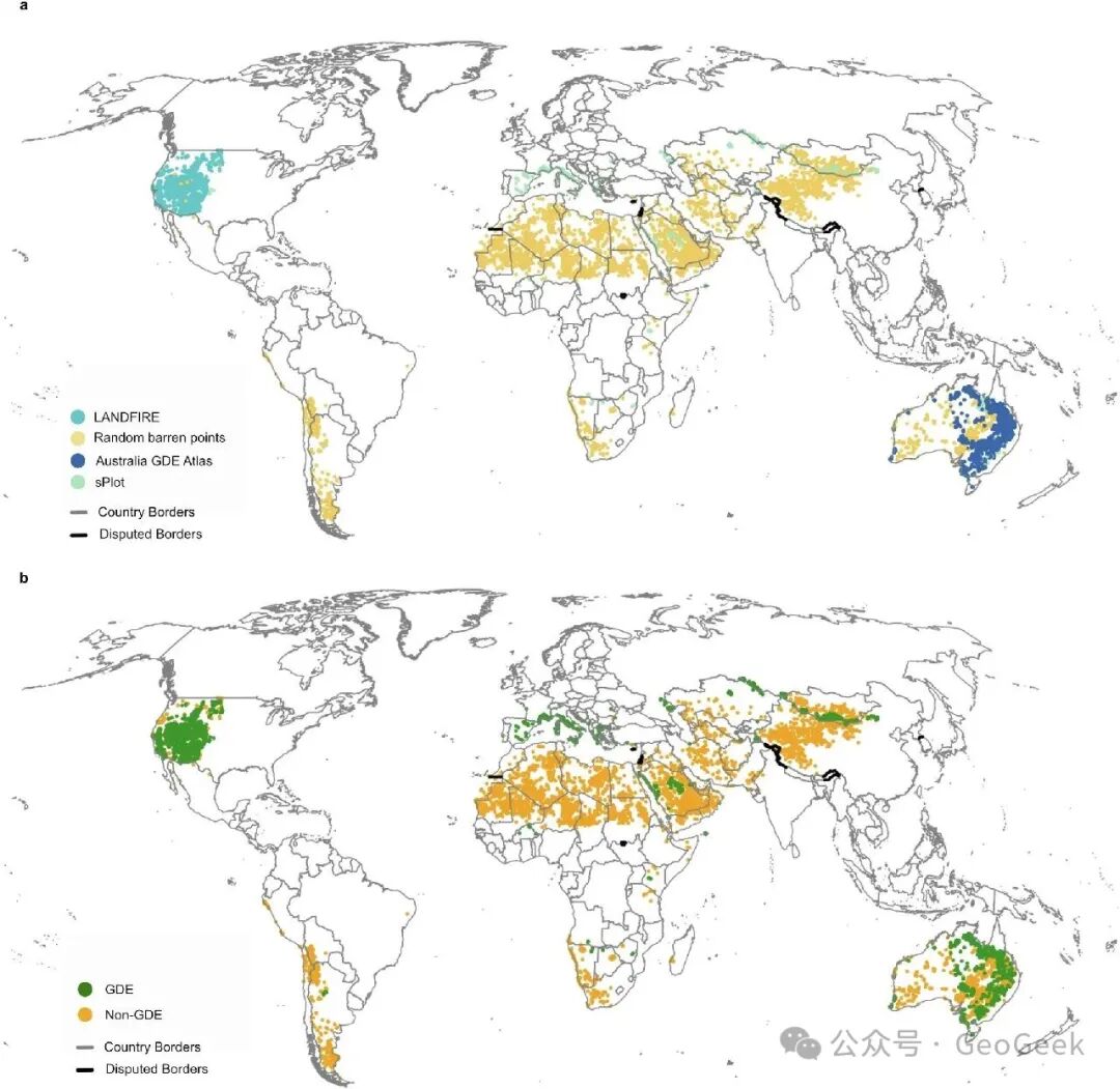
Figure 3 · Spatial distribution of the training data. Rohde et al. (2024, Nature) list the sources and class composition of the GDE training and validation data in Extended Data Fig. 1. For global ecological mapping, the geographic coverage of the training set and the consistency of the label definition can matter more than the apparent completeness of the final map.

This is why a global map can be methodologically misleading even when every pixel is filled. Visually, a continuous surface suggests uniformity, completeness, and equal confidence. In reality, evidential strength may vary greatly across space.

The area of applicability framework proposed by Meyer and Pebesma (2022, Nature Communications) is useful here. The issue is not that Van Nuland or Rohde should not have produced global maps. It is how the products should be read. In regions well supported by training data, they may function as operational information products. In highly extrapolated areas, or where label definitions shift, they are better understood as hypothesis maps or screening layers that indicate where further validation is most needed.

The value of a global map should not be confused with globally uniform reliability.

02 · Temporal extrapolation risk

The temporal version of the problem is especially clear in Miles and Bingham (2024), Progressive unanchoring of Antarctic ice shelves since 1973. A major contribution of the paper is its attempt to extend the evidence for Antarctic ice-shelf thickness change back before the era of satellite altimetry.

The authors are explicit about the evidence chain. Direct satellite-altimetry observations of ice-shelf thickness change begin around 1992. To reach further back, the study uses change in pinning-point area as a proxy for thickness change and extends the record to 1973–1989. It measures pinning-point change in three periods—1973–1989, 1989–2000, and 2000–2022—and “by proxy infer[s] changes to ice-shelf thickness back to 1973–1989.”

This is an ingenious method, not a crude one. But it is also a classic case of temporal transfer: a proxy relation that can be checked more directly in recent decades is used to interpret processes in an earlier period.

The phrase “a fifty-year record” therefore needs to be read carefully. It does not mean fifty years of homogeneous, continuous, direct thickness observations. More precisely, the authors use a proxy relation with partial recent validation together with historical Landsat mosaics to construct a five-decade reconstruction.

The paper describes the limitations of that reconstruction. Early imagery must be mosaicked; the products labelled “1973” and “1989” are assembled from observations spanning several years; early Landsat geolocation over Antarctica is relatively poor and requires manual co-registration; and satellite altimetry itself covers mainly the more recent part of the period.

The most defensible description is therefore proxy-supported reconstruction, not a long direct observational record of the same evidential quality as modern altimetry.

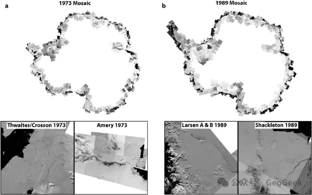
Figure 4 · A nominal time point can conceal a multi-year composite. Extended Data Fig. 1 of Miles and Bingham (2024, Nature) shows Antarctic ice-shelf mosaics labelled 1973 and 1989, while the text explains that both are assembled from Landsat imagery acquired across several years.

Blowes et al. (2019), The geography of biodiversity change in marine and terrestrial assemblages, presents a different temporal problem. It is not temporal transfer in the same sense: the authors do not use recent samples to reconstruct one continuous process decades earlier. The issue is closer to temporal representativeness mismatch.

The study integrates 239 independent studies, largely through BioTIME, and after gridding and filtering analyzes 51,932 local assemblage time series to describe the geography of biodiversity change. The authors explicitly note that the series extend from the late nineteenth century to the present but that most observations come from the past forty years, and that both temporal extent and start date vary substantially. Tropical coverage is also comparatively limited.

The paper seeks a global geography of biodiversity change, but its temporal evidence is not a set of long records with similar length and common start dates. It is an assemblage of local series with heterogeneous duration, origin, and historical coverage.

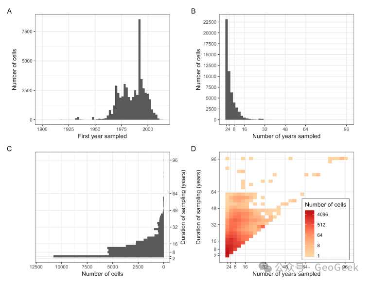
Figure 5 · A global change pattern built from uneven temporal representation. Supplementary Fig. S2 of Blowes et al. (2019, Science) shows the start dates and durations of the included time series. Most are concentrated in recent decades and have limited duration.

The risk is not that the results must be wrong. It is that they are easily over-read as a stable description of “long-term global biodiversity change.” A more exact interpretation is that, within the set of available time series—whose temporal structure is uneven—the analysis identifies regions in which significant richness change or turnover is observed more frequently.

That is not identical to asking where biodiversity has changed most strongly and persistently over a much longer historical period.

Miles and Bingham transfer a more recently testable proxy relation into earlier decades. Blowes et al. aggregate local time series that differ substantially in length and start date into a global spatial comparison. The problems are not the same, but both are forms of temporal representation mismatch.

03 · Reading the boundary of the evidence

Placed together, these four papers reveal a common feature of contemporary global-change research. The most influential work increasingly depends on large aggregated datasets, remote sensing, machine learning, and proxy reconstruction. Such work is often necessary and scientifically valuable. But the parts most readily circulated outside the paper are often the parts most dependent on extrapolation.

A continuous global map can make every pixel look equally trustworthy. A fifty-year historical narrative can make the evidential quality of all fifty years look homogeneous. Neither inference follows from the visual form of the result.

The ambition to ask global-scale questions is not the problem. The default interpretation of the evidence boundary is.

For a global map, we should ask whether the training samples cover the relevant environmental space, whether validation is spatially independent, and whether extrapolated regions are identified. For a multidecadal narrative, we should ask whether the evidence is direct observation, proxy-supported reconstruction, or a synthesis of heterogeneous time series.

The most useful lesson of these Nature and Science papers is therefore not whether any one headline conclusion should be accepted or rejected. It is that when the scale of the conclusion exceeds the scale of the evidence, representation mismatch becomes central to how the result should be read.

References

• Bastin, J.-F. et al. The global tree restoration potential. Science 365, 76–79 (2019).
• Ploton, P. et al. Spatial validation reveals poor predictive performance of large-scale ecological mapping models. Nature Communications 11, 4540 (2020).
• Meyer, H. & Pebesma, E. Machine learning-based global maps of ecological variables and the challenge of assessing them. Nature Communications 13, 2012 (2022).
• Van Nuland, M. E., Averill, C., van den Hoogen, J., et al. Global hotspots of mycorrhizal fungal richness are poorly protected. Nature (2025).
• Rohde, M. M., Albano, C. M., Stella, J. C., et al. Groundwater-dependent ecosystem map exposes global dryland protection needs. Nature 632, 101–107 (2024).
• Miles, B. W. J. & Bingham, R. G. Progressive unanchoring of Antarctic ice shelves since 1973. Nature 626, 785–791 (2024).
• Blowes, S. A., Supp, S. R., Antão, L. H., et al. The geography of biodiversity change in marine and terrestrial assemblages. Science 366, 339–345 (2019).